titanic-gaussian-regression
Gaussian process regression on titanic dataset
Gaussian process regression is a powerful machine learning technique used for various applications, including regression and classification tasks. In this article, we will explore the application of Gaussian process regression on the Titanic dataset. Our goal is to predict the survival status of passengers based on their age and fare.
Dataset
The dataset is from the Titanic prediction competition. We will use the training set which contains data from 891 passengers in a csv format.
Directory
| # | Column | Null | Type | Definition |
|---|---|---|---|---|
| 0 | PassengerId | non-null | int64 | |
| 1 | Survived | non-null | int64 | Survival |
| 2 | Pclass | non-null | int64 | Ticket class, 1 = 1st, 2 = 2nd, 3 = 3rd |
| 3 | Name | non-null | string | |
| 4 | Sex | non-null | string | Gender "male" or "female" |
| 5 | Age | non-null | float64 | Age in years |
| 6 | SibSp | non-null | int64 | # of siblings / spouses aboard the Titanic |
| 7 | Parch | non-null | int64 | # of parents / children aboard the Titanic |
| 8 | Ticket | non-null | string | Ticket number |
| 9 | Fare | non-null | float64 | Passenger fare |
| 10 | Cabin | non-null | string | Cabin number |
| 11 | Embarked | non-null | string | Port of Embarkation, C = Cherbourg, Q = Queenstown, S = Southampton |
Exploration
Let's explore the key metrics of our dataset, with a specific focus on the Age, Fare, and Survived features. Understanding the distribution and statistics of these features can provide valuable insights into the dataset.
Using pandas we can quickly do this using the describe function.
import pandas as pd

df = pd.read_csv("./data/titanic.csv")
df.describe()
This gives us a general description of the dataset.
| Metric | PassengerId | Survived | Pclass | Age | SibSp | Parch | Fare |
|---|---|---|---|---|---|---|---|
| Count | |||||||
| Mean | |||||||
| Standard Dev | |||||||
| Min | |||||||
| 25th %ile | |||||||
| Median (50%) | |||||||
| 75th %ile | |||||||
| Max |
We will briefly discuss the metrics on the features we will later use in the regression.
Passenger Age
- Count: There are 714 non-null entries in the "Age" column, indicating that some passengers have missing age information.
- Mean Age: The average age of passengers is approximately 29.7 years.
- Standard Deviation: The standard deviation is about 14.5, which indicates the spread or variability in passenger ages.
- Minimum Age: The youngest passenger in the dataset is approximately 0.42 years old.
- Median Age (50th Percentile): The median age is around 28 years, meaning that half of the passengers are older than this age, and half are younger.
- Maximum Age: The oldest passenger in the dataset is 80 years old.
Fare
- Mean Fare: The average fare paid by passengers is approximately $32.20.
- Standard Deviation: The standard deviation of fares is approximately $49.69, suggesting a wide range of fare values.
- Minimum Fare: The lowest fare paid is $0.00, indicating that some passengers may have traveled for free.
- 25th Percentile: 25% of passengers paid $7.91 or less for their fare.
- Median Fare (50th Percentile): The median fare is approximately $14.45.
- 75th Percentile: 75% of passengers paid $31.00 or less for their fare.
- Maximum Fare: The highest fare paid is $512.33, indicating significant variation in fare prices.
Survival
- Mean Survival Rate: The average survival rate is approximately 38.4%, indicating that about 38.4% of passengers in the dataset survived.
Normalization and transforming
Before applying Gaussian process regression, we need to prepare the dataset. Luckly the dataset is arelady very consitent, only the following minor steps are necessary.
Column: Sex
Currently is stored in string format. We want to remap that to a integer value.
- "female" => 0
- "male" => 1
Inconsistent entries
To make sure all the entries have a Age, Fare and Sex column we will delete any that do not match that.
We can implement these steps using python and pandas :
# Normalize "Sex"
df.loc[df["Sex"] == "female", "Sex"] = 0
df.loc[df["Sex"] == "male", "Sex"] = 1
df = df.astype({
    "Sex": "int32"
}, errors="ignore")

# Remove inconsistent entries
df = df[df["Age"].notnull()]
df = df[df["Fare"].notnull()]
df = df[df["Sex"].notnull()]

df.info()
Regression
Data preparation
We will use the "Age" and "Fare" columns to predict passenger survival. Let's prepare the data for regression:
X = np.array([df["Age"], df["Fare"]])
X = np.transpose(X)
y = np.array(df["Survived"])
You will notice here that the regression algorithm requires the input data to have a particular shape of
(n_samples, n_features)which we construct using numpy'stransposefunction.
We also need to split the data into training and test sets for evaluation:
from sklearn.model_selection import train_test_split

X_train, X_test, y_train, y_test = train_test_split(X, y, test_size=0.33, random_state=42)
Model
We will use sklern's gaussian process classifier which is based on laplace approximation. We will use RBF also known as squared-exponential as the kernel. Which gives good results using it as a classifier.
from sklearn.gaussian_process import GaussianProcessClassifier
from sklearn.gaussian_process.kernels import RBF

kernel = 1.0 * RBF(1.0)
gpc = GaussianProcessClassifier(kernel=kernel, random_state=0).fit(X_train, y_train)
Results
Evaluation
To evaluate the model's performance we will use log marginal likelihood, accuracy and log-loss.
from sklearn.metrics import accuracy_score, log_loss

print(
    "Log Marginal Likelihood: %.3f"
    % gpc.log_marginal_likelihood(gpc.kernel_.theta)
)
print(
    "Accuracy: %.3f (full dataset) %.3f (test dataset)"
    % (
        accuracy_score(y, gpc.predict(X)),
        accuracy_score(y_test, gpc.predict(X_test))
    )
)
print(
    "Log-loss: %.3f (full dataset)" % log_loss(y, gpc.predict_proba(X)[:, 1])
)
With our model we get the following metrics.
| Matric | Value |
|---|---|
| Log Marginal Likelihood | |
| Accuracy (Full Dataset) | |
| Accuracy (Test Dataset) | |
| Log-loss |
Log Marginal Likelihood
The log marginal likelihood provides insight into the model's fit to the data. In our case, it indicates how well the Gaussian process model fits the given data. A lower log marginal likelihood suggests a better fit. In this scenario, a log marginal likelihood of
Accuracy
Accuracy is a commonly used metric for classification tasks. It measures the proportion of correctly predicted labels in the dataset. In this case, the model achieved an accuracy of approximately
Log-loss
Log-loss is a measure of the accuracy of a probabilistic classifier, and it quantifies how well the predicted probabilities match the true outcomes. A lower log-loss value indicates better performance. In this scenario, a log-loss of
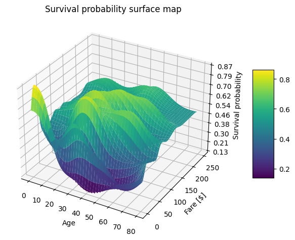
Visualizing survival probabilities
To gain deeper insights into the results obtained from the Gaussian process regression model, we can visualize the survival probability. These visualizations provide a clear representation of how passenger age and fare influence the predicted survival probabilities.
Surface plot
In this visualization, we use passenger Age as the
Heatmap
The heatmap is another valuable visualization that simplifies the understanding of survival probability. In this heatmap, we represent passenger age and fare as coordinates. The color intensity in each cell of the heatmap corresponds to the predicted survival probability for passengers with specific age and fare values.
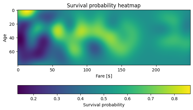
The heatmap provides a two-dimensional representation of the survival probability. It visually emphasizes areas of interest, such as higher survival rates for specific age groups or fare ranges. For instance, it can reveal that children tend to have a higher survival rate, as indicated by brighter regions on the heatmap.
Discussion
The results of our Gaussian process regression model on the Titanic dataset are promising but leave room for further improvement. The accuracy scores, both on the full dataset and the test dataset, indicate that the model is reasonably effective at predicting passenger survival based on age and fare. However, there are several points to consider:
- Feature Selection: Our model used only two features, "Age" and "Fare," for prediction. Exploring additional features, such as "Pclass" or "Embarked," could potentially enhance the model's predictive power.
- Hyperparameter Tuning: Fine-tuning the kernel parameters of the Gaussian process, such as the length scale of the RBF kernel, might lead to improved results. Hyperparameter optimization can be applied to achieve a better fit to the data.
- Data Imbalance: The Titanic dataset may suffer from class imbalance, with more non-survivors than survivors. Techniques like oversampling, undersampling, or the use of different evaluation metrics may help address this issue.
- Model Interpretability: Gaussian process models provide a measure of uncertainty, which can be valuable for decision-making. Understanding and visualizing the uncertainty in predictions can provide additional insights.
In summary, while the Gaussian process regression model shows promise in predicting passenger survival, there are avenues for further exploration and enhancement to achieve even better results. This includes feature engineering, hyperparameter tuning, and addressing class imbalance to create a more robust predictive model.